The first edition of the 12-team College Football Playoff (CFP) is finally upon us! The tournament begins with First Round matchups on December 20^th and 21^st and concludes with the National Championship game on January 20^th in Atlanta. The 12-team bracket, featuring the top five ranked conference champions and seven at-large teams is shown below.

While we’ll have to wait until January 20^th to find out who will raise the trophy, we can use analytics to shed some light on who may be favored to win. Our analytical tool of choice for this situation is Monte Carlo simulation. Monte Carlo simulation is a computational technique that uses random sampling to help us simulate complex systems and see possible outcomes. This method is particularly useful in scenarios where more direct analytical solutions are difficult to develop. Monte Carlo simulation is widely used in fields like finance, engineering, and physics to help model uncertainty and to understand variability.

So how does Monte Carlo simulation work? Let’s look at a simple example: flipping a coin. When we flip a coin, we have two possible results: heads and tails. If the coin is “fair”, we assume that the probability of getting a heads is 0.5 and getting a tails is also 0.5. We’ll assume that heads and tails are the only possible outcomes of a coin flip (ignoring the possibility of the coin ending up on its edge or some other bizarre outcome). All we have to do now is map the outcome probabilities to the number line between 0 and 1. Let’s assign heads to the values between 0 and 0.5 and tails to the values between 0.5 and 1. Note that it doesn’t matter which order we do the mapping (i.e., tails could be mapped from 0 to 0.5, if we wanted). We end up with a number line that looks like the image below.

Probabilities for a Monte Carlo Simulation of Coin Flip

To simulate a coin flip, we then generate a random number between zero and one. This can be done with Excel’s RAND function or can be easily implemented in R or Python. Let’s say we generate a random number value of 0.2875775. What coin flip result does this map to? Because the generated random number is between 0 and 0.5, we would say that the coin flip result is a heads.

Mapping a Random Number to a Simulated Coin Flip Result

We could simulate flipping many coins by generating many random numbers and mapping each to a coin flip result. We can then examine the distribution of coin flip results. For a simulation of 100 coin flips, we might get 53 heads and 47 tails. The next time we simulate 100 coin flips, we might get 59 tails and 41 heads. If you’d like to experiment with a simple coin flip Monte Carlo simulation, check out this demonstration created via Claude (an AI tool).

So, what does all of this have to do with college football simulation? Well, if we have a probability estimate that a team will win a match-up with another team, we can treat the simulation of the game just like a coin flip, but with potential uneven probabilities associated with the outcomes (unless of course our two teams are perfectly, evenly matched). For example, if Team A has a 0.75 probability (75%) to defeat Team B, we simply set up our zero to one number line accordingly. We can then generate random numbers as we did before to simulate the game many times.

Where do we get our probabilities for college football game matchups? We could make our own estimates, or we could use estimates produced by others. For this article, we use the probability estimates provided by Massey Rating’s Matchup tool. This tool allows us to select any two college football teams and then generates probability estimates. We’ll use these probabilities to help us simulate the 2024 College Football Playoff. We can simulate the playoff many times and look at the distribution of results to gain insight into which teams are most likely to win (or not win) the playoff.

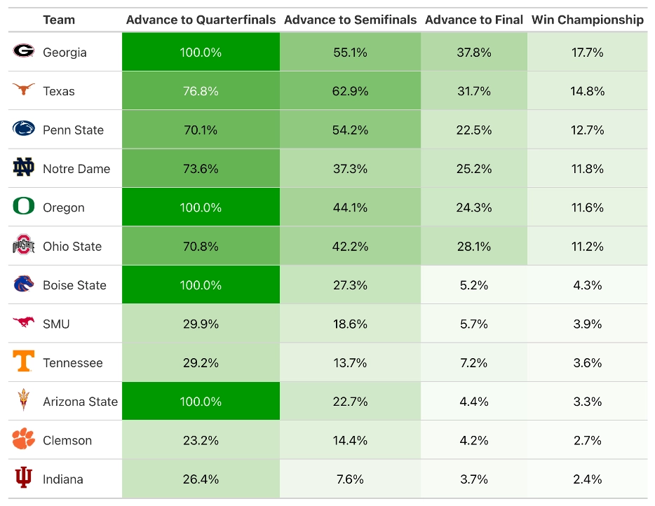
Let’s examine the results of simulating the 2024 College Football Playoff 10,000 times. Note that I’m using the “gt” package for R together with the “cfbplotR” package to produce the results tables and to include team logos. The simulation model suggests that Georgia is a slight favorite to win the championship. Georgia wins the championship in 17.7% of the simulations. Texas, Penn State, Notre Dame, Oregon, and Ohio State all have simulated championship percentages greater than 11%. There is then a significant drop-off with the remaining teams all having chances of less than 5%. It’s notable that two teams (Boise State and Arizona State) that receive byes to the Quarterfinals appear in this group. Perhaps we’ll see modifications to the seeding process in future years to better seed teams by actual strength rather than rewarding conference champions.

Percentage Chance to Advance to Each Round

The next figure shows the National Championship Game match-ups from the simulation runs. Here we see the most frequently occurring match-up is Georgia and Texas facing off for a third time this season.

CFP Finals Simulated Match-ups

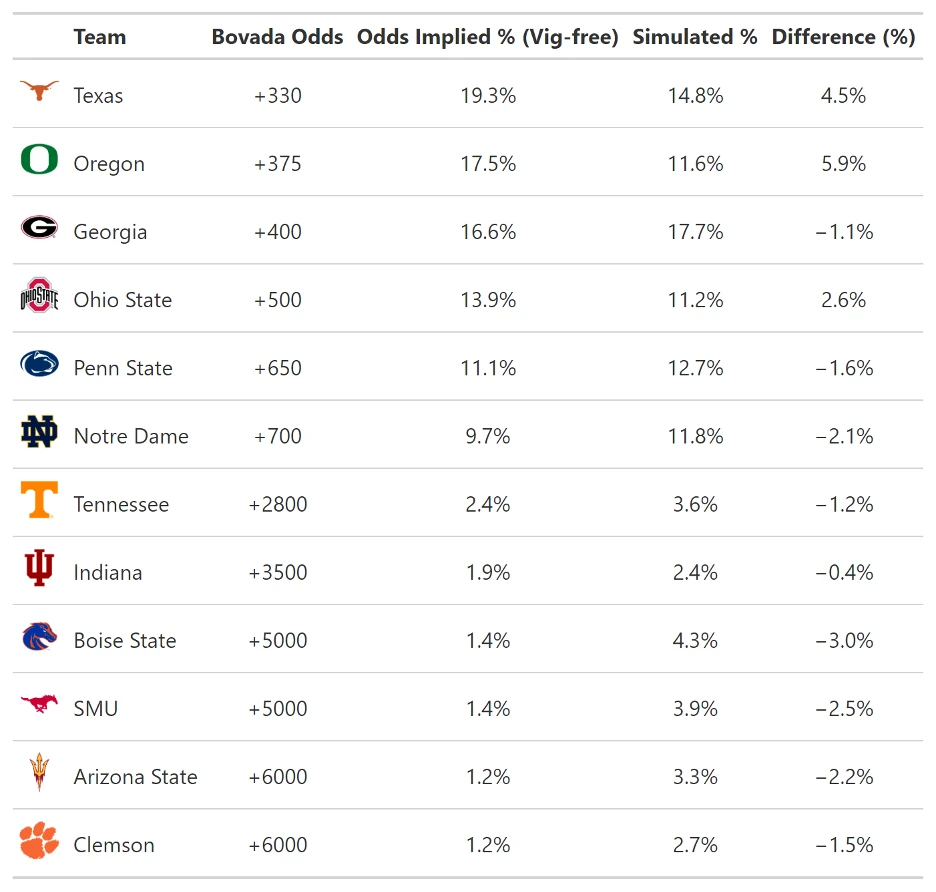
It’s probably worth asking: “Is this simulation model any good?” One way to validate the model would be to compare the simulation model results with results from a different model. For example, how do the probabilities compare to those derived from odds from betting markets? The table below shows the current (as of December 12th) National Championship odds from Bovada. The “Bovada Odds” column expresses the odds for each of the twelve teams to win the National Championship. These odds are given in American-style odds and can be easily converted to implied probabilities. During this conversion, we remove Bovada’s “vig” (i.e., house edge) to get "vig-free” implied probabilities. We can compare the vig-free percentages with the percentages from our simulation model. It looks like our model is pretty good or at least seems to be reasonably well aligned with the betting markets.

Simulation Results versus Betting Odds

Author

Dr. Stephen Hill, Associate Professor of Data Analytics in Samford University's Brock School of Business and the Center for Sports Analytics.